
Hi… This post is about the marvelous feature in MS Excel, the Pivot Table. Pivot Table is the quickest way to summarize the data without using any formula. Now, this is a deep subject and we will try to learn it one step at a time. This part is all about basics. Here we have a sales data file, roughly 100 rows. The link to download this sample file is provided with this article so that you can practice your skills on it.
Follow these steps to get a Pivot Table of your data:
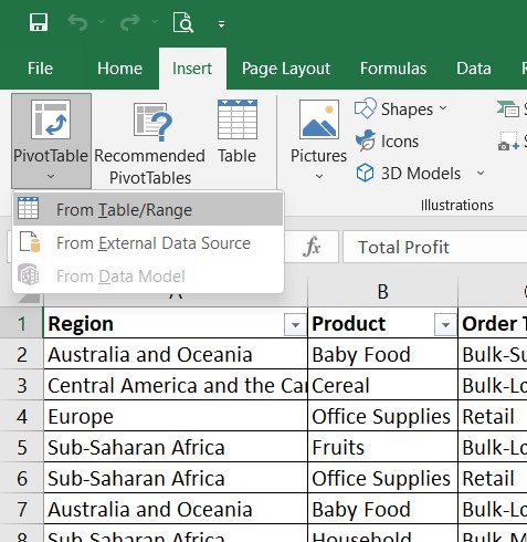
1. Go to Insert>> Pivot Table>> From Table/Range
2. The dialogue box will appear with your range already selected. If not, click on the arrow and select the range manually using Shift + Arrow. Once you select the range, click again on the same arrow button to return to the dialogue box.
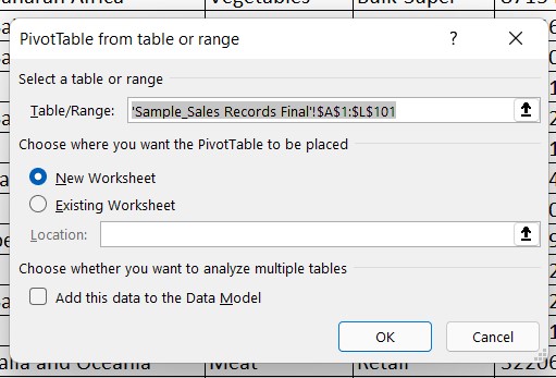
3. Select New Worksheet and click OK
4. A new worksheet with Blank Pivot Table will open.
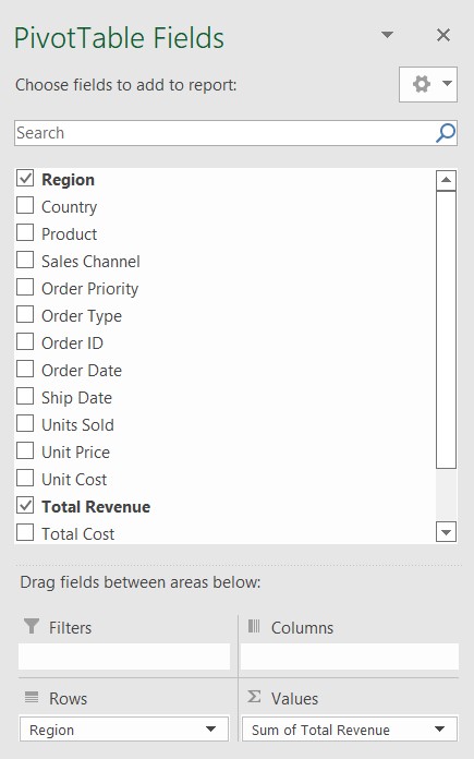
5. To create a summary, go to the Pivot Table Fields.
a. Here we have Table Headers as Fields. We will tick the check box of what we want in the summary.
b.To get the Region-wise Revenue summary, tick the Region and Total Revenue.
c. As you can see, the pivot table has automatically taken the Region in Rows and Total Revenue in Values
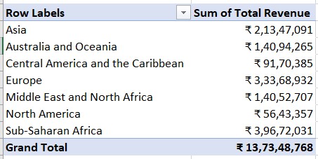
d.Come back to the once blank Pivot Table & you will find the summary ready.
6. The beauty of Pivot Table is that you can modify any item you want and it will automatically update the summary within a fraction of a second.
a. Let’s create a Region-wise Profit Summary
b. Go to Pivot table Fields.
c. Untick the checkbox of Total Revenue and Tick the Box of Total Profit and your summary is updated.
d. Change the formatting of the profit amounts to ‘Currency’ remove the numbers after the decimal point and the summary is ready.
Using these steps, you can create a summary of any data.
Stay tuned for the next part.
If you want to watch how it’s done, please check this Instagram Post.
Link to download the Sample Sales File.